
RootBasicTutorial
Introduction
This tutorial will cover the basic usage of ROOT for the purpose of running analysis tools on ATLAS data.Starting ROOT
To provide a common environment, we will start ROOT from lxplus (If you don't have an lxplus account, see WorkBookGetAccount):- Windows:
- Need PuTTy, Exceed/cygwin installed. See: Connecting to unix computers
- For Cygwin/X installation instructions, see: Installing Cygwin/X and Starting Cygwin/X in the Cygwin/X User's Guide.
- Unix:
ssh -X lxplus.cern.ch
Once inside lxplus, we will need to tell our environment where ROOT is
located. This is normally done by the Athena initialization scripts
(i.e source setup.sh) but since we won't run Athena we need to do this manually (or put in your profile). In lxplus prompt write:
export ROOTSYS=/afs/cern.ch/sw/lcg/external/root/5.21.02/slc4_ia32_gcc34/root
export LD_LIBRARY_PATH=$ROOTSYS/lib:$LD_LIBRARY_PATH
export PATH=$ROOTSYS/bin:$PATH
root
You should see the ROOT splash screen, followed by the ROOT prompt:
 *******************************************
  *                                         *
  *        W E L C O M E  to  R O O T       *
  *                                         *
  *   Version  5.18/00d       29 May 2008   *
  *                                         *
  *  You are welcome to visit our Web site  *
  *          http://root.cern.ch            *
  *                                         *
  *******************************************

ROOT 5.18/00d (branches/v5-18-00-patches@24036, Jun 02 2008, 10:09:00 on linux)

CINT/ROOT C/C++ Interpreter version 5.16.29, Jan 08, 2008
Type ? for help. Commands must be C++ statements.
Enclose multiple statements between { }.
root [0]
Quit ROOT:
root [1] .q
Make your own local directory for the tutorial:
mkdir rootTut
cd rootTut
Copy the tutorial files into this directory:
cp ~nir/public/rootTutorial/* .
C++ Basics
We will introduce the C++ absolute essentials needed to understand and write ROOT code.Variable declaration
In C++ the user must first define their variables before using them. There exists several variable types:int, long, float, double, char, bool ..... To define variables:
int myInt; double myDouble=3.14; //Variable's value initialize to 3.14 char myChar='c'; bool myBool = true; |
// clause is used for commenting the rest of the line.
Function declaration
Function is a short block of code needed to be called various times with different parameters. Functions, as variables can have types. A function's type is the type of the variable which the function returns. To define functions:int myFunction (int x, int y) {
int sum = x + y;
cout << "x + y = " << sum << endl;
return sum;
} |
{ and } clauses define the block of code that belongs to the function.cout is used to print out content of variables or strings. To call the function:
int z; z = myFunction( 1, 2 ); |
Conditions
if ( ( x > 10 && y < 20 ) || z == 30 ) {
    // do something
} else {
    // do something else
} |
== operator is the equal-to operator (not to be confused with = which is the assignment operator). The
&& and || operators are logical AND and logical OR operators.
Loops
Loops perform a certain code several times. They begin by initializing the control variable to a certain value, defining a stop condition to the loop, then declaring how to increment the control variable:for (int i=0; i<20; i++) {
//do something
} |
Arrays
Arrays are a collection of same-type variables bound together by a common name. To declare an array of 10 integers:int myArray[10]; |
Accessing an array's element is done via:
myArray[4] (for the 5th element).
Sometimes it is not clear prior to running the program how many elements an array requires. For example, when running your analysis code, you will not know for certain how many muons are in your event until runtime. For this reason it is possible to dynamically set the size of arrays during runtime. This requires a different syntax than the one we've just discussed. We will cover this when we talk of dynamic variable allocation.
Pointers
Pointers are a very tricky concept to comprehend in C++. A pointer is a variable like any other, but its content is the memory address to another variable. For example:int myInt = 5; // Define a variable whose content is 5 int* p_myInt; // Define a pointer to an int variable p_myInt = &myInt; // Assign the memory address of myInt (&myInt) to p_myInt. cout<<myInt<<endl; // prints out 5 cout<<p_myInt<<endl; // prints out 0x80ec118 - the memory address of myInt cout<<*p_myInt<<endl; // prints out 5 - the content of the variable to which p_myInt points to |
& operator is called the reference operator and gives the memory address to a variable.The
* operator is called the dereference operator and gives the content of the variable to which a pointer points to.Try this in ROOT.
For more information see: Pointers
Automatic vs. Dynamic variable allocation
When declaring a variable in C++, certain amount of bytes (depending on the type of the variable) are set aside for it in the computer memory. This memory is reserved for the content of this variable. There are two ways in which such memory allocation can be done:Automatic allocation: Also known as stack allocation. This is the usual way in which memory is reserved when declaring variables (e.g.
int myInt;). When a program begins, or when a function is accessed, its variables are reserved a place in an area of memory (called the stack).
When the program or the function ends, the variables declared in it
lose scope and their allocated space on the stack is automatically
deallocated. This means that after the scope of the
program/function/code block in which the variable was declared, one
cannot access it any longer.Example:
int globVar = 5;
int* p_locVar;
if (globVar > 0) {
    //Inside the scope of the if block {}
    int locVar = globVar*2;
    p_locVar = &locVar;
    cout<<globVar<<endl; // Prints 5;
    cout<<locVar<<endl; // Prints 10;
    cout<<*p_locVar<<endl; // Prints 10;
} // Leaving the scope of the if block, locVar memory is freed
cout<<globVar<<endl; // Prints 5
cout<<locVar<<endl; // ERROR. locVar is not declared in this scope
cout<<*p_locVar<<endl; // ERROR. The address p_locVar points to is no longer reserved (contains a random value) |
locVar declared within the block has been automatically destroyed once exiting the block. Any pointers pointing to it (like p_locVar) are now pointing to an area of memory which may contain anything (that area of memory it is no longer reserved to locVar).
Dynamic allocation: Also known as heap
allocation. Automatic allocation works well for most variables, but
there are cases in which it is not enough. Such cases occur when data
is needed to be accessed outside the scope in which it was created in,
or memory needs to be reserved for variables on the fly during
run-time. For this reason, dynamic variable allocation was invented.
The memory-allocation for dynamic variables is done in a different area
of memory (called the heap) and is controlled
entirely by the user. Once declared the memory reserved for these
variables will not be deallocated until either the user deallocates it
directly or the program ends.
Example:
int globVar = 5;
int* p_locVar;
if (globVar < 0) {
    //Inside the scope of the if block {}
    int* locVar = new int (globVar*2);
    p_locVar = locVar;
    cout<<globVar<<endl; // Prints 5
    cout<<*locVar<<endl; // Prints 10
    cout<<*p_locVar<<endl; // Prints 10
} // Leaving the scope of the if block
cout<<globVar<<endl; // Prints 5
cout<<*locVar<<endl; // ERROR. locVar pointer is not declared in this scope. A copy of the address it contained is in p_locVar
cout<<*p_locVar<<endl; // Prints 10
delete p_locVar; // Freeing the memory reserved for locVar earlier |
locVar
is created dynamically and therefore the memory reserved for it will
not be released when leaving the block (like previous example).
However, locVar itself will be destroyed once leaving the block, hence it is essential to save its address in some global pointer (p_locVar) to be accessed outside the block.
For more information see: Stack vs Heap Allocation
Classes
A class is an expanded concept of a data structure: instead of holding only data, it can hold both data and functions. An object is an instantiation of a class. Think of a class as a blueprint; an object is the actual item(s) that have been built using this blueprint. In terms of variables, a class would be the type, and an object would be the variable. Classes is a lengthy topic in C++ and as such will be discussed very briefly in this tutorial - just enough to understand and use in ROOT.class MyClass {
public:
int m_x;
void print() { cout<<"m_x="<<m_x<<endl;}
}; |
To use this class:
MyClass classExample; // Declares an object of type MyClass classExample.m_x = 5; // Assigns a value to variable x inside classExample classExample.print(); // Calls the print function inside classExample |
Classes customarily have constructor functions. A constructor
function is a function that is called right at the creation of the
class object and is used to initialize the various member variables of
the class.
For example, in ROOT:
TH1 hist("h_eta", "Eta Distrubition", 100, -3., 3.); |
- The 1st value initializes the name of the histogram
- The 2nd initializes its title
- The 3rd initializes the number of bins for this histogram
- The 4th and 5th values initialize the lower and upper edges of this histogram.
ROOT
Basics
Interperter vs. Compiler
An interpreter takes a program (or a command line) and runs it by examining each instruction, turning it into machine language, executing it (possibly showing its results) and continuing to the next instruction. This is in contrast to a compiler which turns the entire program into machine language before executing it. A compiled program takes a while to compile, but when it is compiled, it runs about 10 times faster than an interpreted one. For this reason, one uses a compiled program when they need to make a program once, then run it many times without changes. But when a short, interactive program is required and is being built together gradually, one uses ROOT interpreted program (or macros).ROOT uses CINT as its C++ interpreter, allowing interactive user interaction via a simple command-line user interface.
ROOT command-line
CINT commands start with ".":root[] .? //this command will list all the CINT commands root[] .L <filename> //load [filename] root[] .x <filename> //load and execute [filename] root[] .q // quits ROOT root[] .qqqqq // REALLY quits ROOT |
Shell commands start with ".!":
root[] .! ls |
root[] .! cat macroName.C |
cat is the Unix command to dump the content of a file to stdout.
C++ commands follow C++ syntax:
root[] TBrowser *b = new TBrowser() |
Tab-completion also works in CINT:
root[] TLine *l = new TL<TAB> |
<TAB> means pressing the TAB key)
Macros
A ROOT macro file is any file (usually .C) containing a set of ROOT/C++ instructions for ROOT to run. Macros are run in the ROOT interperter, which means that each line is being interpreted sequentially by CINT and (for unnamed macros) the objects created are later accessible via the ROOT command line.There are two kinds of macros: unnamed macros and named macros:
- named macros are macros with a full function
definition on the first line of the macro. The function name must be
identical to the macro file name.
myMacro.C:
Due to the nature of C, all the objects defined within a named macro are destroyed once the macro finishes running and the function loses scope (unless the objects were dynamically declared).void myMacro(int param1, int param 2) { ... // list of commands }
Named macros are often used when one needs to pass parameters to your macro, or when one needs multiple functions to be called inside the macro. - unnamed macros are macros without a function definition, so they cannot take any input parameter or have multiple functions defined in them.
myMacro.C:
All the objects created within an unnamed macro are left in memory once the macro ends, so one can pick them up and manipulate them even after the macro is done. This makes unnamed macros the common way to run short scripts within ROOT. However, it also means that it is important to remove these objects before each call to the macro, so they won't be reused and hence produce unexpected results. To do this, you can just put a call to{ ... // list of commands }gROOT->Reset();in the beginning of each unnamed macro.
Histograms
Simple histogram
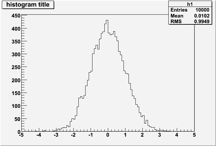
Creating 1-,2- and 3D histograms in ROOT is a very simple task: [histGaus.C].Load and execute the [histGaus.C] macro:
root[] .x histGaus.C |
root[] .! emacs histGaus.C & |
{
  TH1F h1 ("h1", "histogram title", 100, -5.0 , 5.0);  // Create a 1D histogram object of floats
  // Filling up histogram with random events:
  TRandom rGen (0); // Creates a random number generator object with seed 0
  for (int i=0; i<10000; i++) { // Repeat 10000 times
    float x = rGen.Gaus(0.0, 1.0); // Generate a random number according to the gaus distribution with mean=0, sigma=1
    h1.Fill(x); // Fill the histogram with x
  }
  h1.Draw(); // Draw the histogram onto the screen
} |
TH1F constructor take are: - Object name: This is the internal name by which ROOT will recognize this object.
- Histogram title: This will show up as the title of the histogram when it is drawn
- Number of bins
- Leftmost edge of the histogram
- Rightmost edge of the histogram
Result:
The same thing can be done in a more concise way by doing: [histGaus2.C]
{
    TH1F h2 ("h2", "histogram title", 100, -5.0 , 5.0);  // Create a 1D histogram object of floats
    h2.FillRandom("gaus",10000); // Calls the FillRandom function of the TH1F class which fills the histogram with 10000 gaus-distributed events
    h2.Draw(); // Draw the histogram
} |
Creating 2- and 3D histograms is done similarly: [histGaus3.C]
{
  TH2F h3 ("h3", "histogram title", 100, -5.0 , 5.0, 200, 0.0, 1.0);  // Create a 1D histogram object of floats
  TF2 func ("gaus2","xgaus(0)*ygaus(3)"); // Create a 2-param gaussian distribution function
  // Set the parameters of the function we created:
  func.SetParameters(1. , 0., 1.,    // Set the parameters of the first gaussian to N=1, mean=0, sigma=1
		     1. , 0.5, 0.1); // Set the parameters of the second gaussian to N=1, mean=0.5, sigma=0.1
  h3.FillRandom("gaus2",1000000); // Calls the FillRandom function of the TH1F class which fills the histogram with 10000 gaus-distributed events
  gStyle->SetPalette(1); // Sets a better-looking color-palette than the default ROOT one
  h3.Draw("COLZ"); // Draw the histogram
} |
This code creates a 2D (TH*2*F) histogram with 100 x
bins in range (-5,5) and 200 y bins in range (0,1). It then declares a
2D function according to which the random variables are going to be
selected. Then it fills the histogram with random variables according
to the declared function and draws it.
Let's look in detail into each line:
-
TH2F h3 ("h3", "histogram title", 100, -5.0 , 5.0, 200, 0.0, 1.0);: Declares aTH2Fobject with name, title, xbinx, xrange, ybins, yrange -
TF2 func ("gaus2","xgaus(0)*ygaus(3)");: Declares aTF2(2-variable function) object with the name "gaus2" and the equation "xgaus(0)*ygaus(3)" (equivalent to![$ P_{0}\cdot exp^{-\frac{[(x-P_{1})/P_{2}]^2}{2}} \cdot P_{3}\cdot exp^{-\frac{[(y-P_{4})/P_{5}]^2}{2} $](RootBasicTutorial_files/latexb834e96699611e5517508fef4cf2319e.png) ). 0 and 3 represent the place of the first parameter of this function in the following line.
). 0 and 3 represent the place of the first parameter of this function in the following line.
-
func.SetParameters(1. , 0., 1.,1. , 0.5, 0.1);: Sets the parameter of this function. The function had 6 parameters, P0-2 belong to xgaus, P3-5 belong to ygaus -
h3.FillRandom("gaus2",1000000);: Fills the histogram with 1000000 events distributed according to a function called "gaus2" which we created earlier -
h3.Draw("COLZ");: Draws the histogram
Try right-clicking on the histogram in different places and playing with the different menu items. For example, try changing values in "SetLineAttributes" menu.
Manipulating properties
Different properties of the histogram can be changed prior or post draw. For example:- Changing a histogram title:
h.SetTitle("my new title"); - Setting axis title:
h.SetXTitle("my X axis title");
Or less concisely:h.GetXaxis()->SetTitle("my X axis title");
GetAxis()calls the histogram's GetAxis function which returns the histogram's axis. ThenSetTitle("")calls the axis' SetTitle function which sets the title for the axis. - Changing the axis range:
h.SetAxisRange(-1,1,"X");
After this is called, one need to update the canvas on which the hist is drawn on to see the change. This is usually done by:c1.Modified(); c1.Update();which tells the canvasc1that its contents was modified, then updates it. - Scaling a histogram:
h.Scale(10);
For a complete set of changeable properties (and much more) see class TH1 in the ROOT reference guide.
Histogram stacks
It is also possible to stack two histograms together: [histStack.C]{
gROOT->Reset(); // Resets the ROOT environment
THStack hs("hs","test stacked histograms"); // Define the histogram stack object
// Setting the histograms:
TH1F *h1 = new TH1F("h1","test hstack",100,-4,4); // Dynamically create a new histogram
h1->FillRandom("gaus",20000); // Fill histogram
h1->SetFillColor(kRed); // Set histogram fill color to red
h1->SetFillStyle(3001);
hs.Add(h1); // Add histogram to the histogram stack object
TH1F *h2 = new TH1F("h2","test hstack",100,-4,4);
h2->FillRandom("expo",15000);
h2->SetFillColor(kBlue);
h2->SetFillStyle(3001);
hs.Add(h2);
TH1F *h3 = new TH1F("h3","test hstack",100,-4,4);
h3->FillRandom("landau",10000);
h3->SetFillColor(kGreen);
h3->SetFillStyle(3001);
hs.Add(h3);
// Printing the histograms:
TCanvas c1("c1","stacked hists", 10, 10, 1000, 500); // Create a canvas, setting the position to (10,10) and size to (1000,500)
c1.Divide (3); // Divide the canvas in 3
c1.cd(1); // Go to the first pane of the canvas
hs.Draw(); // Draw the histogram stack with the histograms stacked on top of each other
c1.cd(2); // Go to the second pane of the canvas
hs->Draw("NOSTACK"); // Draw the histogram stack without stacking
c1.cd(3); // Go to the third pane of the canvas
hs.Draw("PADS"); // Draw the histogram stack with the histograms stacked on top of each other
} |
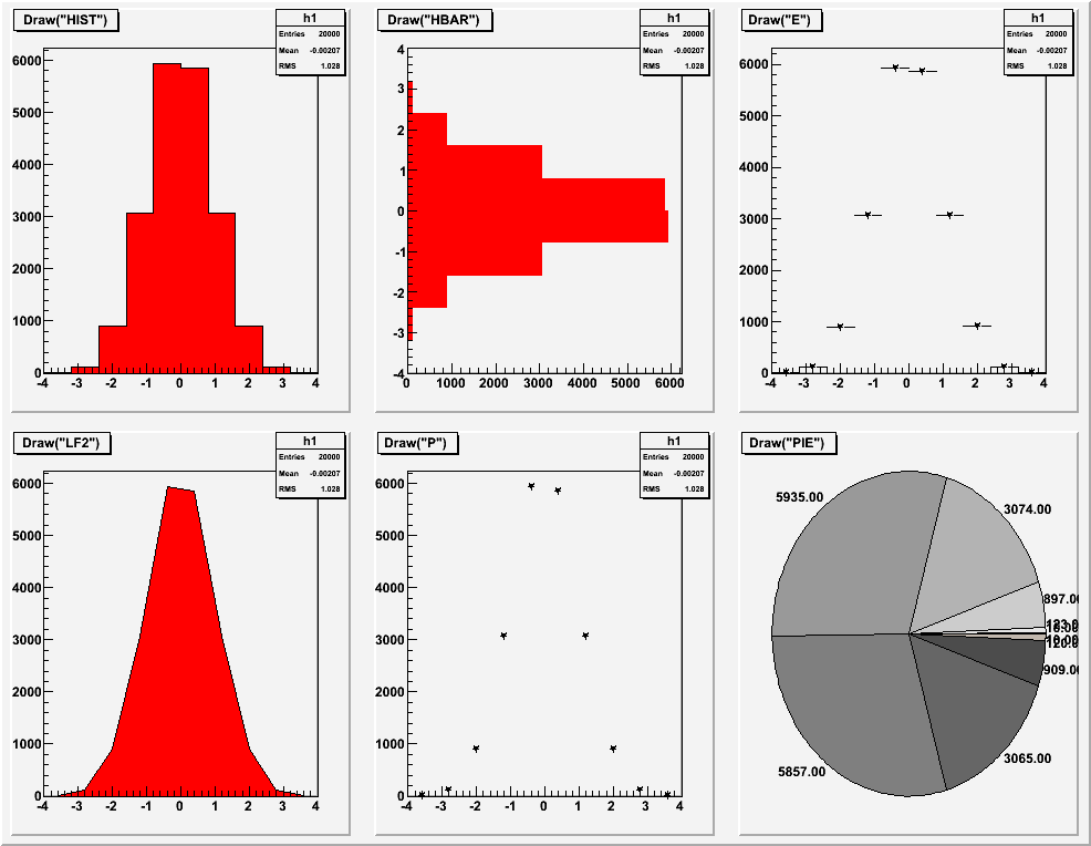
Draw options
ROOT Histograms support many draw options accessible by calling theDraw() function with draw parametersFor 1D histograms: [histDraws.C]
For 2D histograms: [histDraws2.C]
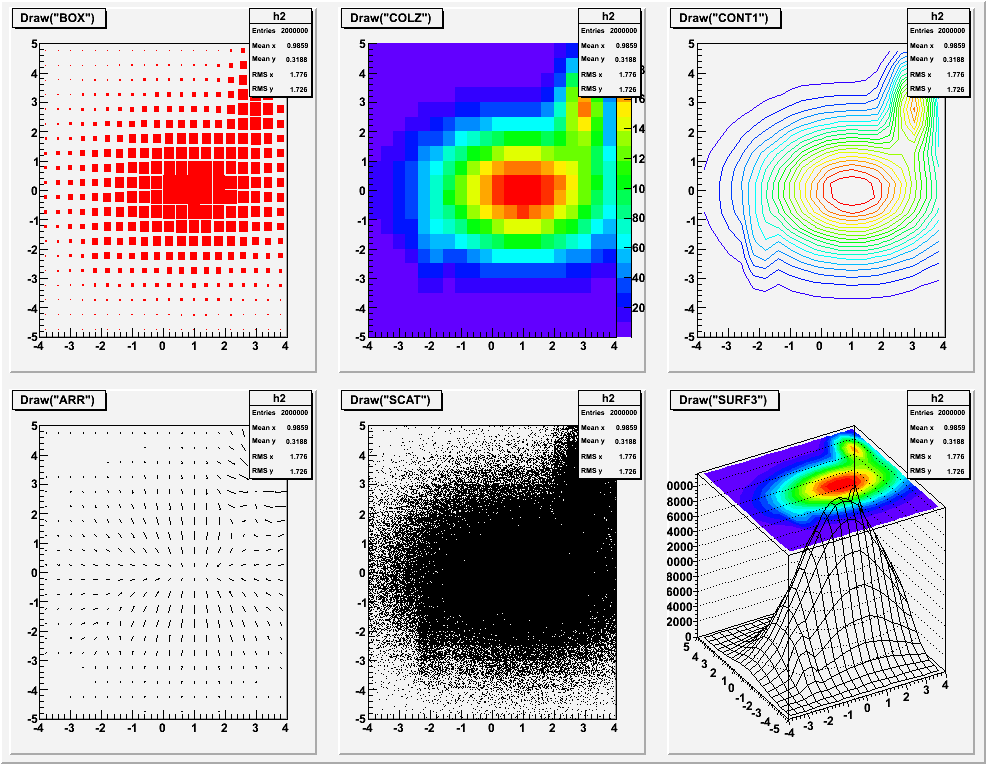
For a complete list, see: Histogram's plotting options in THistPainterClass
For more examples of possible histogram styles, see: Histogram examples in THistPainter class (notice you can switch between picture and the source used to draw it)
Legend
Graph and histogram legends are also available via the ROOT classTLegend. A legend is merely a block which contains the graph/histogram style (fill color, line color, marker color) and a text label.
To create one, simply call the TLegend constructor: TLegend legend(xMin, yMin, xMax, yMax); with: -
xMin/yMinbeing the position of the lower left corner of the legend block (in pad coordinates, i.e. between 0 and 1) -
xMax/yMaxbeing the position of the higher top corner of the legend block (in pad coordinates, i.e. between 0 and 1)
To add an entry to a legend, we will use the AddEntry method:
legend.AddEntry(object, "Entry name") - which reads the style of the object to the legend entry whose name is in ""
For a detailed documentation of the TLegend class, see: TLegend class
We will revisit the stacked histogram example and add a legend to it: [legends.C]
{
  gROOT->Reset(); // Resets the ROOT environment
  THStack hs("hs","test stacked histograms"); // Define the histogram stack object
  // Setting the histograms:
  TH1F *h1 = new TH1F("h1","test hstack",100,-4,4); // Dynamically create a new histogram
  h1->FillRandom("gaus",20000); // Fill histogram
  h1->SetFillColor(kRed); // Set histogram fill color to red
  h1->SetFillStyle(3001);
  hs.Add(h1); // Add histogram to the histogram stack object
  TH1F *h2 = new TH1F("h2","test hstack",100,-4,4);
  h2->FillRandom("expo",15000);
  h2->SetFillColor(kBlue);
  h2->SetFillStyle(3001);
  hs.Add(h2);
  TH1F *h3 = new TH1F("h3","test hstack",100,-4,4);
  h3->FillRandom("landau",10000);
  h3->SetFillColor(kGreen);
  h3->SetFillStyle(3001);
  hs.Add(h3);
  /***************************************************/
  // Make the legend:
  TLegend legend(0.6,0.7,0.99,0.99); // Dimensions of the legend block
  // Adds legend entries:
  legend.AddEntry(h1, "Gaussian");
  legend.AddEntry(h2, "Exponential");
  legend.AddEntry(h3, "Landau");
  /***************************************************/
  // Printing the histograms:
  TCanvas c1("c1","stacked hists", 10, 10, 1000, 500); // Create a canvas, setting the position to (10,10) and size to (1000,500)
  c1.Divide (3); // Divide the canvas in 2
  c1.cd(1); // Go to the first pane of the canvas
  hs.Draw(); // Draw the histogram stack with the histograms stacked on top of each other
  legend.Draw(); // Draws the legend
  c1.cd(2); // Go to the second pane of the canvas
  hs->Draw("NOSTACK"); // Draw the histogram stack without stacking
  legend.Draw(); // Draws the legend
  c1.cd(3); // Go to the third pane of the canvas
  hs.Draw("PADS"); // Draw the histogram stack with the histograms stacked on top of each other
  legend.Draw(); // Draws the legend
} |
Fitting
Histogram and graph fitting is done in ROOT via theFit method:
hist.Fit(function, "fitOptions", "drawOptions", lowRange, hiRange); |
- function can be either the name of the function you want to fit to or the function object itself: e.g.
- Explicitly write the function inside the Fit method:
hist.Fit("[0]*x+[1]*sin(x)", "", "", 0, 10);... doesn't work for me (Stephen Haywood; 23-Dec-08) - Define TF1 function object first, then send it to the Fit method:
TF1 func("myFunction","[0]*x+[1]*sin(x)", 0, 10); // Define TF1 function object
hist.Fit("myFunction","","",0,0); // Send function *name* to the Fit method. range [0,0] means fit the entire range
hist.Fit(&func,"","",0,0); // Send *a pointer* to the func object to the fit method
- Explicitly write the function inside the Fit method:
- fitOptions is a list of fitting options:
"W" Set all weights to 1 for non empty bins; ignore error bars
"WW" Set all weights to 1 including empty bins; ignore error bars
"I" Use integral of function in bin instead of value at bin center
"L" Use Loglikelihood method (default is chisquare method)
"LL" Use Loglikelihood method and bin contents are not integers)
"U" Use a User specified fitting algorithm (via SetFCN?)
"Q" Quiet mode (minimum printing)
"V" Verbose mode (default is between Q and V)
"E" Perform better Errors estimation using Minos technique
"B" Use this option when you want to fix one or more parameters and the fitting function is like "gaus","expo","poln","landau".
"M" More. Improve fit results
"R" Use the Range specified in the function range
"N" Do not store the graphics function, do not draw
"0" Do not plot the result of the fit. By default the fitted function is drawn unless the option"N" above is specified.
"+" Add this new fitted function to the list of fitted functions (by default, any previous function is deleted)
"C" In case of linear fitting, don't calculate the chisquare (saves time)
"F" If fitting a polN, switch to minuit fitter
Options can be chained together. e.g."QML"for a quiet, improved fit using logliklihood method - drawOptions are similar to the histogram drawing options discussed here
- lowRange,*hiRange* are the ranges of the fit.
A fitted histogram would look like this: [histFit.C]
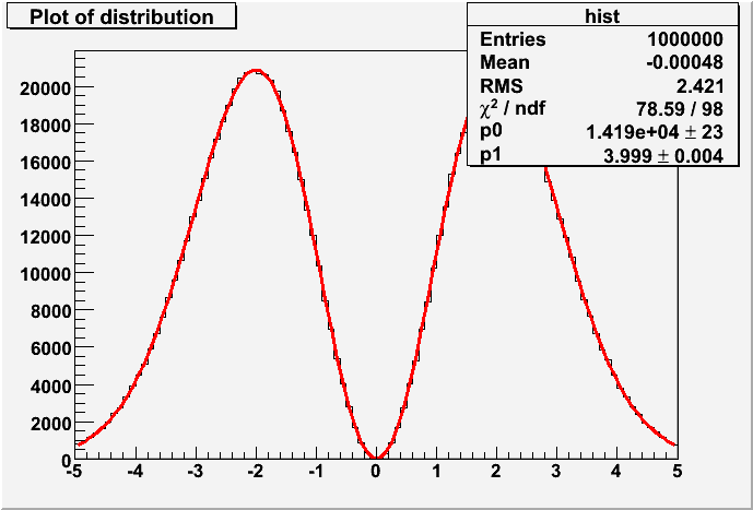
For a detailed documentation of the Fit method, see: TH1:Fit
Exercise 1
Draw a histogram with random events distributed according to the formula: with
with  and fit it.
Working with files
ROOT allows easy access to files for reading/writing data. The ROOT class in-charge of ROOT files is calledTFile (see: TFile).tutorial.root.
Opening files
To open a ROOT file, simply do:TFile myFile("filename.root", option);
option tells ROOT how to open the file.
If option = -
"NEW"or"CREATE"create a new file and open it for writing, if the file already exists the file is not opened. -
"RECREATE"create a new file, if the file already exists it will be overwritten. -
"UPDATE"open an existing file for writing. if no file exists, it is created. -
"READ"open an existing file for reading (default).
"" (default), READ is assumed.
So to open a file for reading do: TFile myFile("filename","READ");
![]() Make sure that you close
the file before your program is finished. Large number of open files
that have not been closed might cause ROOT to crash and the file to be
corrupted.
Make sure that you close
the file before your program is finished. Large number of open files
that have not been closed might cause ROOT to crash and the file to be
corrupted.
To close a file, do: myFile.Close();
![]() NOTE:
Once a file is closed, all objects that were read from it lose scope
and can no longer be accessed (so if you opened a file, read a
histogram from it and printer it to screen, once the file closes, the
histogram will disappear). If you wish to avoid that and read an object
to memory, you will need to clone it.
NOTE:
Once a file is closed, all objects that were read from it lose scope
and can no longer be accessed (so if you opened a file, read a
histogram from it and printer it to screen, once the file closes, the
histogram will disappear). If you wish to avoid that and read an object
to memory, you will need to clone it.
Try it with the tutorial.root file.
Getting objects from files
After opening a file, it is possible to get objects that were previously saved to this file (histogras, trees, graphs, etc'). First, to see what objects the file contains, do:myFile.ls(); |
For example, we will look at the tutorial.root file:
root [0] TFile myFile("tutorial.root","READ")
root [1] myFile.ls()
TFile**         tutorial.root
 TFile*         tutorial.root
  KEY: TTree    Muon;1  Muon
You can see a TTree object called "Muon" inside the file.
To get a certain object from a file you need to use the Get method:
myFile.Get("objectName"); |
Try it with the tutorial.root file.
Notice that ROOT returns a line similar to:
(class TObject*)0x216b6e0
This means that the command we issued (Get) returns a pointer (*) to object TObject. You may wonder why we get a TObject back instead of a TTree, which is the real type of the object in the file. To ensure ROOT works generically on all types of objects, the Get method returns a pointer to a generic TObject object (TObject is the parent object from which all ROOT objects are derived from). TObject objects have the most basic functionality shared between all ROOT objects. To make sure the returned object is a TTree (and as such has all the functionality of TTree s) one needs to statically cast the returned object to its real type type. This is done like this:
root [0] (TTree*) myFile.Get("Muon");
(class TTree*)0x216b6e0
We see here that we get a TTree pointer back.
To assign this returned value to a variable so we can use it later, do:
TTree* muonTree = (TTree*) myFile.Get("Muon");
This will allow us to use muonTree later on.
![]() In newer versions of ROOT the static cast is done automatically to the
object it is assigned to. Still, it is good practice to do it
explicitly.
In newer versions of ROOT the static cast is done automatically to the
object it is assigned to. Still, it is good practice to do it
explicitly.
Writing objects to files
Writing objects to file is done with theWrite method:
myObject.Write(); |
The name of the object in the file will be the same as the name given to the object. If you wish to write the object under a different name, use
myObject.Write("objectNameInFile");
Subdirectories in files
Sometime it is useful to have objects saved in dedicated sub-directories inside a file (e.g. a sub-directory for the file's histograms and another for the file's trees).- To create a subdirectory in a file, do:
myFile.mkdir("subdirName"); - To access this subdirectory, do:
myFile.cd("subdirName");
Once the subdirectory has been accessed, subsequent objects written to this file will be written into this subdirectory. - To read an object from a subdirectory, simply prepend the name of the subdirectory to the objectname:
myFile.Get("subdirName/objectName"); - To list the content of a subdirectory, do:
myFile.GetDirectory("subdirName")->ls();
Exercise 2
Edit your previous code from Exercise 1 to write the histogram data into a file. Reset ROOT variables (gROOT->Reset()) and try to read the histogram back from the file and print it.
TGraph
TBrowser
While most of the time you will work with ROOT via the command-line and macro interfaces, ROOT also has a GUI interface called TBrowser. Using a TBrowser one can browse all ROOT objects, manipulate them and draw them.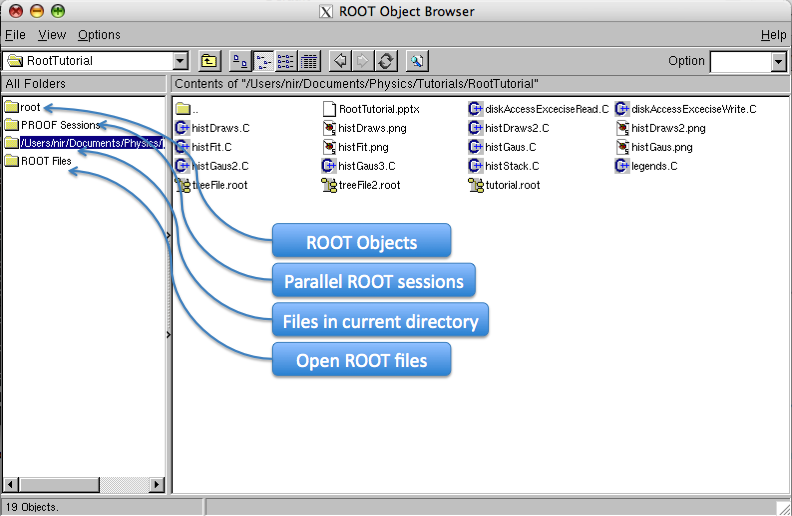
TBrowser is somewhat buggy and has a very limited functionality, but it serves to have a general overview over files and their objects, especially when they are big and complex.
To call TBrowser, do:
TBrowser myTBrowser;This creates an object called
myTBrowser and opens the TBrowser GUI window.
TTrees
TTree s are the main physics-analysis objects in ROOT. A TTree
is a container of measured quantities with simple interfaces to plot,
cut, filter, cross-correlate and write the data it contains. It can be
optimized to reduce disk-space or enhance access speed.A
TTree is basically a long table containing a variety of different objects. Each column in this table is called a branch, while each line is an entry.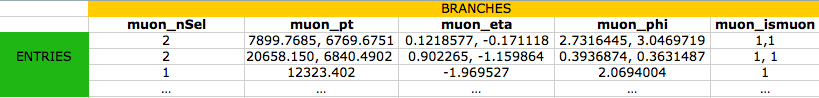
A branch can contain a single variable, an array, or a complex object.
For example, in the table above, muon_pt, muon_eta, muon_phi and
muon_ismuon are all arrays containing the values of the n muons measured for each event (entry). The number of muons found in the event in specified by muon_nParticle.
![]() TTrees are meant to be write-once read-many sort of objects. After a
tree is written and closed, it is not recommended (though possible) to
add branches/entries to it. The recommended way add more data is to
create a new tree in a new file and "chain" the two files together
using TChain.
However, this will not be covered in this tutorial. You can find more
information in the "Chains" subsection of the Trees chapter in the ROOT Users Guide.
TTrees are meant to be write-once read-many sort of objects. After a
tree is written and closed, it is not recommended (though possible) to
add branches/entries to it. The recommended way add more data is to
create a new tree in a new file and "chain" the two files together
using TChain.
However, this will not be covered in this tutorial. You can find more
information in the "Chains" subsection of the Trees chapter in the ROOT Users Guide.
TTrees are incredibly versatile and many things that can be accomplished with trees will not be covered in this tutorial. It is highly recommended to read the TTree section in the ROOT Users Guide. For more information, see the TTree class
TreeViewer
Similar toTBrowser,
TreeViewer is a GUI for tree handling. It is a quick and easy way to
examine a tree and also learn how to plot tree branches in
command-line. To open a TreeViewer do
tree.StartViewer();. For example, for our tutorial.root file:
{
    TFile myFile("tutorial.root","READ");
    TTree *myTree = (TTree*) myFile.Get("Muon");
    myTree->StartViewer();
    myFile.Close(); // AFTER you have examined file with TreeViewer
} |
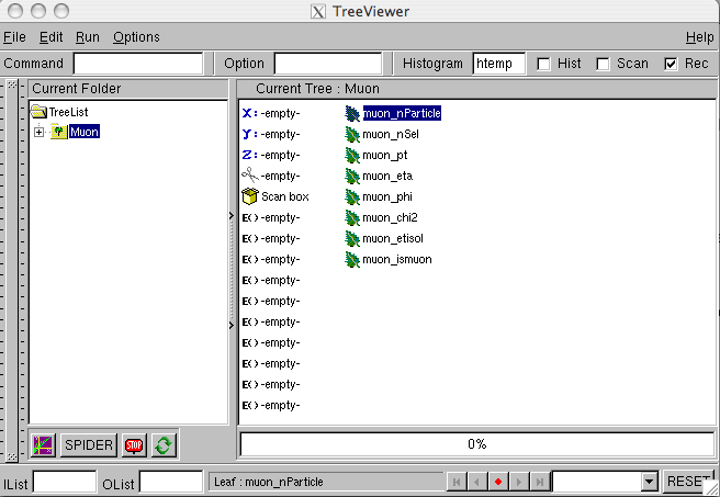
Each branch in the tree is shown as a leaf.
- Double-clicking a branch plots its distribution.
- To draw a correlation plot of one variable against the other, drag each branch to the respected axis (
X:andY:in TreeViewer) and click the Draw button (button in TreeViewer with a small graph - bottom left). - To perform a cut on a variable, drag it to the cut (scissors) icon, then right-click it and click EditExpression to specify the cut.
- It is possible to plot complex formulas based on the quantities in the branches. To do this, right-click the
E()icons and click EditExpression, then specify the formula.
Notice that the Rec checkbox on the top right of the
window is ticked. This means that whatever you do in the TreeView is
recorded and can be reviewed later in the command-line. This is a great
learning tool as it lets you see different ways to use tree->Draw().
After you you succeed to do a complex plot using the GUI, you can look
it up in the command-line and copy it to your macro, instead of
repeating the same process in the GUI every time you want to plot it.
![]() Take some time to go through the different menus/options for the TreeView window.
Take some time to go through the different menus/options for the TreeView window.
Print and Scan
We will now leave the GUI and concentrate solely on the command-line interface.Another good way to overview the contents of your tree is using
Print and Scan.
- Print Print gives you verbose information about the structure of your tree table (branches). To use it, do:
myTree->Print();
The output would look like this:****************************************************************************** *Tree :Muon : Muon * *Entries : 2750 : Total = 616365 bytes File Size = 233741 * * : : Tree compression factor = 1.94 * ****************************************************************************** *Br 0 :muon_nParticle : muon_nParticle/I * *Entries : 2750 : Total Size= 11688 bytes One basket in memory * *Baskets : 0 : Basket Size= 32000 bytes Compression= 1.00 * *............................................................................* *Br 1 :muon_nSel : muon_nSel/I * *Entries : 2750 : Total Size= 11658 bytes One basket in memory * *Baskets : 0 : Basket Size= 32000 bytes Compression= 1.00 * *............................................................................* *Br 2 :muon_pt : * *Entries : 2750 : Total Size= 103382 bytes File Size = 34244 * *Baskets : 2 : Basket Size= 32000 bytes Compression= 1.63 * *............................................................................*
In red you see the name of the tree, followed by the number of entries for this tree. After the tree data, specific branch information is given, starting with the name of the branch, then the type of variable the branch holds (Imeans integer. For a complete list of branch variable types, see "Case A" in ROOT TTree reference).
- Scan Scan gives a table-like view of the content of specified branches. To use it, do:
myTree->Scan();. If you are only interested in specific branches, give them in a colon-separated list:myTree->Scan("muon_nPar:muon_nSel:muon_pt");The output ofmyTree->Scan()looks like this:*********************************************************************************************************************** * Row * Instance * muon_nPar * muon_nSel * muon_pt * muon_eta * muon_phi * muon_chi2 * muon_etis * muon_ismu * *********************************************************************************************************************** * 0 * 0 * 2 * 2 * 7899.7685 * 0.1218577 * 2.7316445 * 0 * 6291.3779 * 1 * * 0 * 1 * 2 * 2 * 6769.6751 * -0.171118 * 3.0469719 * 0.3129153 * 6490.0097 * 1 * * 1 * 0 * 2 * 2 * 20658.150 * -0.902265 * 0.3631487 * 1.5234277 * 8323.7158 * 1 * * 1 * 1 * 2 * 2 * 6840.4902 * -1.159864 * 0.3936874 * 0.4210140 * 7002.5869 * 1 *
Note that the same row (entry) repeats several times. This is due to the array of values in muon_pt, muon_eta, etc'.
Drawing TTree branches
We have seen how the content of branches can be drawn using the TreeView GUI. Now we will see how to do it in command-line.Drawing tree branches is done via the
Draw method:
myTree->Draw("branchName(s)", "selection", "draw options", number_of_entries, first_entry); |
-
"branchName(s)"is the branch name you want to draw. To draw a correlation plot of one branch against the other, do:"first_branch:second_branch". -
"selection"is the cuts you want to apply to your plot. For example:"param_1 == 1 && param_2 < 0.5". -
"draw options"is the conventional histogram drawing options (specified here). -
number_of_entriesis the number of entries you would like to plot. The default is all, so this is rarely used. -
first entryis the first entry you want to start drawing from. The default is 0, so this is rarely used.
Look at these examples: [treeDraw.C]
{
  gROOT->Reset();
  gStyle->SetPalette(1); // Set the "COLZ" palette to a nice one

  TFile  myFile("tutorial.root"); // Open the file
  TTree* myTree = (TTree*) myFile.Get("Muon"); // Get the Muon tree from the file

  // Draw examples:
  TCanvas c1; // Open a new canvas
  myTree->Draw("muon_pt"); // Simple draw of the muon_pt parameter

  TCanvas c2; // Open a new canvas
  myTree->Draw("muon_pt", "muon_nSel==2"); // Apply a cut to the draw

  TCanvas c3; // Open a new canvas
  myTree->Draw("muon_pt", "muon_nSel==2", "C"); // Apply draw options (smooth curve)

  TCanvas c4; // Open a new canvas
  // Plot eta vs. phi correlation:
  //   "PSR"  - plot using Pseudorapidity/Phi coordinates (X axis is phi)
  //   "COLZ" - A box is drawn for each cell with a color scale varying with contents
  myTree->Draw("muon_eta:muon_phi", "muon_nParticle>0 && muon_chi2<1", "PSR COLZ");

  TCanvas c5; // Open a new canvas
  // Plot pT of first[0] versus the pT of second[1] muon divided by the combined pt
  //   "BOX" - A box diagram
  myTree->Draw("muon_pt[0]/(muon_pt[0]+muon_pt[1]):muon_pt[1]/(muon_pt[0]+muon_pt[1])", "muon_nParticle==2", "BOX");

  TCanvas c6; // Open a new canvas
  c6.SetGrid();  // Plot a grid on this canvas
  // Dump the contents of the draw into a histogram for future manipulation:
  //   "goff" - Do not plot to the screen, just dump to histogram
  myTree->Draw("muon_pt/1000>>h_pt", "muon_pt<60000", "goff");
  // Manipulate the histogram:
  h_pt->SetFillColor(kGreen); // Set fill color
  h_pt->SetTitle("P_{T} distribution"); // Set histogram title
  h_pt->SetXTitle("P_{T} [GeV]"); // Set the X title
  gStyle->SetOptFit(1); // Draw the fit parameters on the histogram
  h_pt->Fit("landau"); // Fit to a landau distribution
  h_pt->Draw(); // Draw the histogram

  myFile.Close(); // Close file
} |
For more information of tree drawing methods, see the "TTree::Draw Examples" in the TTree section of the ROOT Users Guide.
Exercise 3
Plot the invariant mass of the first two muons to identify what the dataset is.
Reading TTrees
TTree::Draw() is good for most of the simple cases you'll
encounter, but sometime you will find you need to run on the actual
tree data for your analysis.
We will look at a simple example of how to read TTree s directly, even though this example can easily be implemented using Draw as well.
[readTree.C]
{
  gROOT->Reset();

  TFile  myFile("tutorial.root"); // Open the file
  TTree* myTree = (TTree*) myFile.Get("Muon"); // Get the Muon tree from the file

  // Preparing the containers to be filled with data from the tree:
  int              muon_nParticle; // Number of muons in an entry
  vector<double>*  muon_pt;        // An array of the pT values for each of the muons
  vector<double>*  muon_eta;       // An array of the eta vlues for each of the muons
  vector<double>*  muon_phi;       // An array of the phi vlues for each of the muons

  // Linking the local variables to the tree branches
  myTree->SetBranchAddress("muon_nParticle", &muon_nParticle);
  myTree->SetBranchAddress("muon_pt",        &muon_pt);
  myTree->SetBranchAddress("muon_eta",       &muon_eta);
  myTree->SetBranchAddress("muon_phi",       &muon_phi);
  // After this stage the local variables are still empty.
  // With every subsequent call to myTree->GetEntry(i) the local variables
  // will be filled with the content of branches

  // Create a histogram with 100 bins between 0-100000 to be filled later:
  gROOT->cd(0); // This tells ROOT to create next object in memory and not in file
  TH1D h("h_muon_pt", "Muon P_{T} histogram",20, 0, 20000);
  gStyle->SetOptStat(111111); // Tells ROOT to list histogram overflow/underflow

  // Loop over all entries in the tree
  //   for each entry, print the pt values and fill them to a histogram
  int nEntries = myTree->GetEntries(); // Get the number of entries in this tree
  for (int iEnt = 0; iEnt < nEntries; iEnt++) {
    myTree->GetEntry(iEnt); // Gets the next entry (filling the linked variables)

    cout<<"Entry #"<< iEnt << endl;
    for (int iPar = 0; iPar < muon_nParticle; iPar++) {
      cout<<"    muon_pt["<< iPar <<"] = "<< muon_pt->at(iPar) << endl;
      h.Fill(muon_pt->at(iPar));
    }
  }
  h.Draw(); // Draw histogram

  myFile.Close(); // Close file
} |
Writing TTrees
Writing trees is done similarly to reading trees:[writeTree.C]
{
  gROOT->Reset();
  // Open the file for writing
  TFile f("treeFile.root","RECREATE");
  // Define the tree
  TTree* myTree = new TTree("bonsai", "tree title");

  // Define auxilary variaqbles:
  Double_t x;
  Double_t y;
  Double_t z;

  // Create tree branches:
  //   this will link the addresses of x, y, z variables to the content of the branch
  //   so that every file myTree->Fill() is called, the content of x,y,z is filled
  //   into a new entry in the tree.
  myTree->Branch("a", &x, "a/D");  // Create a branch called a, linked to local variable x, of type D (double)
  myTree->Branch("b", &y, "b/D");
  myTree->Branch("c", &z, "c/D");

  Int_t n=100000;   // Number of entries to fill
  TRandom rGen(0);  // Create the random number generator
  // Loop over n entries and fill the tree:
  for (Int_t i=0; i < n; i++) {
    x = rGen.Gaus(0.0, 1.0); // Generate a gaussian-distributed random number
    y = x * 5. + 1.;
    z = x + rGen.Gaus(0.0, 0.1);
    // Fills tree:
    myTree->Fill();
  }
  cout<<"Entries in tree: "<<myTree->GetEntries()<<endl;

  // Write tree to file:
  myTree->Write("", TObject::kOverwrite);
  // Close file:
  f.Close();
} |
![]() The rule of thumb for writing verbose DAQ code is to write down every
quantity that you produce to a tree. This way, when something goes
wrong with the DAQ, it is very easy to understand where the problem
occurred just by looking at the produced trees. Also, when you are
later required to extend the DAQ analysis (to produce more plots, for
instance), you can be sure that all the quantities are already written
down and there's no need to rewrite the DAQ code. It's just a matter of
plotting them.
The rule of thumb for writing verbose DAQ code is to write down every
quantity that you produce to a tree. This way, when something goes
wrong with the DAQ, it is very easy to understand where the problem
occurred just by looking at the produced trees. Also, when you are
later required to extend the DAQ analysis (to produce more plots, for
instance), you can be sure that all the quantities are already written
down and there's no need to rewrite the DAQ code. It's just a matter of
plotting them.
MakeClass
When trees are long and complex, as is often the case, writing the code to read them directly is long and error-prone. For this purpose theMakeClass function was introduced to TTree. MakeClass creates a skeleton analysis code for the tree.myTree.MakeClass("filename", "options");
MakeClass takes two parameters: - The base name (no suffix) of the files to be creates for the skeleton analysis.
- General options string (often "").
Loop
which loops over all tree entries and does nothing. Whatever
functionality you wish to implement in the tree reading phase should go
into the Loop function.
Open the tutorial.root file, get the Muon tree, and run its MakeClass? function.
Let's look at the results:
myMuon.h:
//////////////////////////////////////////////////////////
// This class has been automatically generated on
// Mon Oct 20 08:44:13 2008 by ROOT version 5.18/00
// from TTree Muon/Muon
// found on file: tutorial.root
//////////////////////////////////////////////////////////

#ifndef myMuon_h
#define myMuon_h

#include <TROOT.h>
#include <TChain.h>
#include <TFile.h>

class myMuon {
public :
   TTree          *fChain;   //!pointer to the analyzed TTree or TChain
   Int_t           fCurrent; //!current Tree number in a TChain

   // Declaration of leaf types
   Int_t           muon_nParticle;
   Int_t           muon_nSel;
   vector<double>  *muon_pt;
   vector<double>  *muon_eta;
   vector<double>  *muon_phi;
   vector<double>  *muon_chi2;
   vector<double>  *muon_etisol;
   vector<long>    *muon_ismuon;

   // List of branches
   TBranch        *b_muon_nParticle;   //!
   TBranch        *b_muon_nSel;   //!
   TBranch        *b_muon_pt;   //!
   TBranch        *b_muon_eta;   //!
   TBranch        *b_muon_phi;   //!
   TBranch        *b_muon_chi2;   //!
   TBranch        *b_muon_etisol;   //!
   TBranch        *b_muon_ismuon;   //!

   myMuon(TTree *tree=0);
   virtual ~myMuon();
   virtual Int_t    Cut(Long64_t entry);
   virtual Int_t    GetEntry(Long64_t entry);
   virtual Long64_t LoadTree(Long64_t entry);
   virtual void     Init(TTree *tree);
   virtual void     Loop(); // The Loop method running over all entries
   virtual Bool_t   Notify();
   virtual void     Show(Long64_t entry = -1);
};

#endif

#ifdef myMuon_cxx
myMuon::myMuon(TTree *tree)
{
// if parameter tree is not specified (or zero), connect the file
// used to generate this class and read the Tree.
   if (tree == 0) {
      TFile *f = (TFile*)gROOT->GetListOfFiles()->FindObject("tutorial.root");
      if (!f) {
         f = new TFile("tutorial.root");
      }
      tree = (TTree*)gDirectory->Get("Muon");

   }
   Init(tree);
}

myMuon::~myMuon()
{
   if (!fChain) return;
   delete fChain->GetCurrentFile();
}

Int_t myMuon::GetEntry(Long64_t entry)
{
// Read contents of entry.
   if (!fChain) return 0;
   return fChain->GetEntry(entry);
}
Long64_t myMuon::LoadTree(Long64_t entry)
{
// Set the environment to read one entry
   if (!fChain) return -5;
   Long64_t centry = fChain->LoadTree(entry);
   if (centry < 0) return centry;
   if (!fChain->InheritsFrom(TChain::Class()))  return centry;
   TChain *chain = (TChain*)fChain;
   if (chain->GetTreeNumber() != fCurrent) {
      fCurrent = chain->GetTreeNumber();
      Notify();
   }
   return centry;
}

void myMuon::Init(TTree *tree)
{
   // The Init() function is called when the selector needs to initialize
   // a new tree or chain. Typically here the branch addresses and branch
   // pointers of the tree will be set.
   // It is normally not necessary to make changes to the generated
   // code, but the routine can be extended by the user if needed.
   // Init() will be called many times when running on PROOF
   // (once per file to be processed).

   // Set object pointer
   muon_pt = 0;
   muon_eta = 0;
   muon_phi = 0;
   muon_chi2 = 0;
   muon_etisol = 0;
   muon_ismuon = 0;
   // Set branch addresses and branch pointers
   if (!tree) return;
   fChain = tree;
   fCurrent = -1;
   fChain->SetMakeClass(1);

   fChain->SetBranchAddress("muon_nParticle", &muon_nParticle, &b_muon_nParticle);
   fChain->SetBranchAddress("muon_nSel", &muon_nSel, &b_muon_nSel);
   fChain->SetBranchAddress("muon_pt", &muon_pt, &b_muon_pt);
   fChain->SetBranchAddress("muon_eta", &muon_eta, &b_muon_eta);
   fChain->SetBranchAddress("muon_phi", &muon_phi, &b_muon_phi);
   fChain->SetBranchAddress("muon_chi2", &muon_chi2, &b_muon_chi2);
   fChain->SetBranchAddress("muon_etisol", &muon_etisol, &b_muon_etisol);
   fChain->SetBranchAddress("muon_ismuon", &muon_ismuon, &b_muon_ismuon);
   Notify();
}

Bool_t myMuon::Notify()
{
   // The Notify() function is called when a new file is opened. This
   // can be either for a new TTree in a TChain or when when a new TTree
   // is started when using PROOF. It is normally not necessary to make changes
   // to the generated code, but the routine can be extended by the
   // user if needed. The return value is currently not used.

   return kTRUE;
}

void myMuon::Show(Long64_t entry)
{
// Print contents of entry.
// If entry is not specified, print current entry
   if (!fChain) return;
   fChain->Show(entry);
}
Int_t myMuon::Cut(Long64_t entry)
{
// This function may be called from Loop.
// returns  1 if entry is accepted.
// returns -1 otherwise.
   return 1;
}
#endif // #ifdef myMuon_cxx |
myMuon.C
#define myMuon_cxx
#include "myMuon.h"
#include <TH2.h>
#include <TStyle.h>
#include <TCanvas.h>

void myMuon::Loop()
{
//   In a ROOT session, you can do:
//      Root > .L myMuon.C
//      Root > myMuon t
//      Root > t.GetEntry(12); // Fill t data members with entry number 12
//      Root > t.Show();       // Show values of entry 12
//      Root > t.Show(16);     // Read and show values of entry 16
//      Root > t.Loop();       // Loop on all entries
//

//     This is the loop skeleton where:
//    jentry is the global entry number in the chain
//    ientry is the entry number in the current Tree
//  Note that the argument to GetEntry must be:
//    jentry for TChain::GetEntry
//    ientry for TTree::GetEntry and TBranch::GetEntry
//
//       To read only selected branches, Insert statements like:
// METHOD1:
//    fChain->SetBranchStatus("*",0);  // disable all branches
//    fChain->SetBranchStatus("branchname",1);  // activate branchname
// METHOD2: replace line
//    fChain->GetEntry(jentry);       //read all branches
//by  b_branchname->GetEntry(ientry); //read only this branch
   if (fChain == 0) return;

   Long64_t nentries = fChain->GetEntriesFast();

   Long64_t nbytes = 0, nb = 0;
   for (Long64_t jentry=0; jentry<nentries;jentry++) {
      Long64_t ientry = LoadTree(jentry);
      if (ientry < 0) break;
      nb = fChain->GetEntry(jentry);   nbytes += nb;
      // if (Cut(ientry) < 0) continue;
      // HERE GOES YOUR CODE
   }
} |
For more information see: MakeClass function in ROOT reference guide
Exercise 4
Read the tree we've just produced from thetreeFile.root file and plot its variables. Look at correlation plots and use various cuts. Fit the distribution of each of the variables.
Major updates:
-- NirAmram - 09 Sep 2008
Responsible: NirAmram
Last reviewed by: Examples worked through by StephenHaywood - 24 Dec 2008
 Show attachments (7)
 Hide attachments (7)
| I | Attachment | Action | Size | Date | Who | Comment |
|---|---|---|---|---|---|---|
| | TBrowser.png | manage | 94.5 K | 23 Sep 2008 - 15:25 | NirAmram | |
| | TreeTable.png | manage | 23.7 K | 23 Sep 2008 - 18:11 | NirAmram | |
| | TreeViewer.png | manage | 23.1 K | 24 Sep 2008 - 08:57 | NirAmram | |
| | histDraws.png | manage | 24.5 K | 22 Sep 2008 - 08:34 | NirAmram | |
| | histDraws2.png | manage | 64.9 K | 22 Sep 2008 - 08:35 | NirAmram | |
| | histFit.png | manage | 16.5 K | 22 Sep 2008 - 08:35 | NirAmram | |
| | histGaus.png | manage | 10.2 K | 22 Sep 2008 - 08:32 | NirAmram |
|
|
Ideas, requests, problems regarding TWiki? Ask a support question or Send feedback